Programming Tools in Data Science

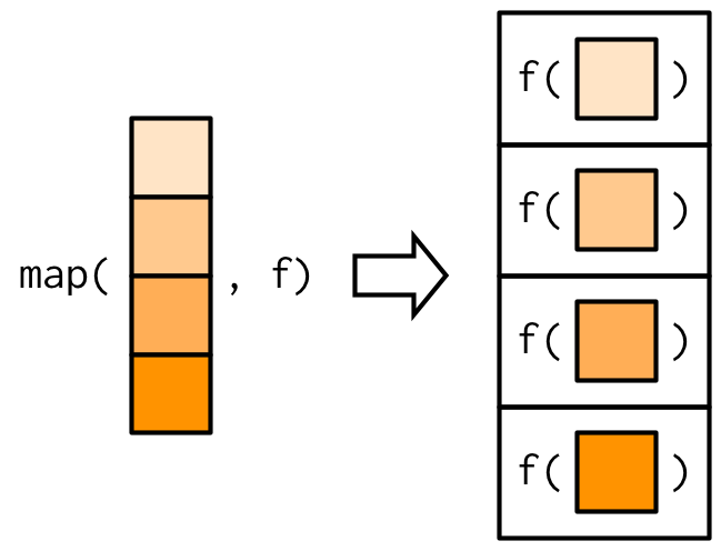
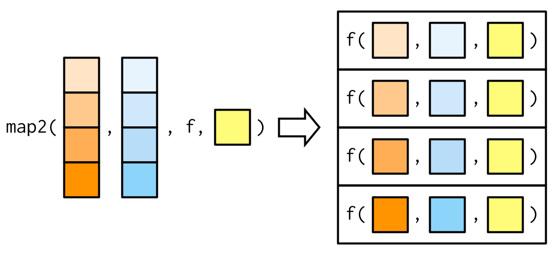
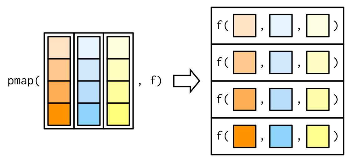
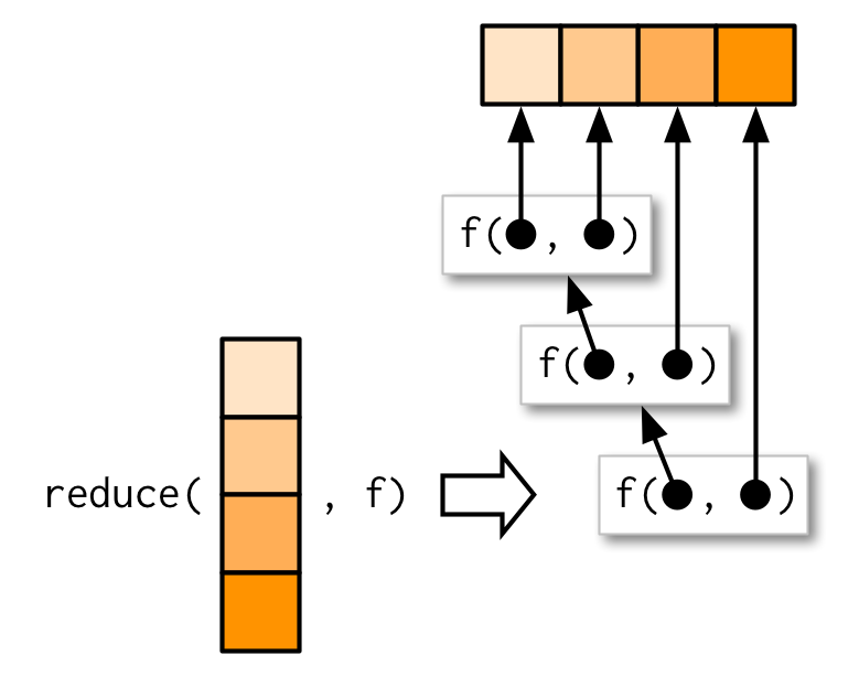
class: center, middle, inverse, title-slide

.title[
# Programming Tools in Data Science
]
.subtitle[
## Lecture #10: Functional programming
]
.author[
### Samuel Orso
]
.date[
### 31 October 2024
]

---

# S3 OOP system
* Object-oriented programming (OOP) is one of the most popular programming paradigm. 
* The type of an object is a **class** and a function implemented for a specific class is a **method**.
* It is mostly used for **polymorphism**: the function interface is separated from its implementation. In other words, the function behaves differently according to the class.
* This is related to the idea of **encapsulation**: the object interface is separated from its internal structure. In other words, the user doesn't need to worry about details of an object. Encapsulation avoids spaghetti code (see [Toyota 2013 case](http://archive.wikiwix.com/cache/index2.php?url=https%3A%2F%2Fwww.usna.edu%2FAcResearch%2F_files%2Fdocuments%2FNASEC%2F2016%2FCYBER%2520-%2520Toyota%2520Unintended%2520Acceleration.pdf)).
* `R` has several OOP systems: S3, S4, R6, ...
* S3 OOP system is the first R OOP system, it is rather informal (easy to modify) and widespread.

---
# Functional programming
* Functional programming is a programming paradigm that generally means writing computer programs by following strict rules, using simple functions (*pure*) that don't change things around (*immutability*, or no side effects).
* Benefits are more maintainable, predictable, and scalable (parallel) code.
* There are several key concepts, including:  
   + *Pure* function: always produces the same output for the same input and has no side effects.
   + *First-class* function: like any other data structure, functions can be passed as arguments to other functions, returned from other functions, and assigned to variables.
   + *Higher-order* function: functions that take one or more functions as arguments or return them as results.

---
# Pure function
* A pure function always produces the same output for the same input.
* Is `rnorm` a *pure* function?

``` r
set.seed(123)
rnorm(10)
```

```
##  [1] -0.56047565 -0.23017749  1.55870831  0.07050839  0.12928774  1.71506499
##  [7]  0.46091621 -1.26506123 -0.68685285 -0.44566197
```

---
# Pure function
* A pure function always produces the same output for the same input.
* Is `rnorm` a *pure* function?

``` r
set.seed(123)
rnorm(10)
```

```
##  [1] -0.56047565 -0.23017749  1.55870831  0.07050839  0.12928774  1.71506499
##  [7]  0.46091621 -1.26506123 -0.68685285 -0.44566197
```

``` r
set.seed(124)
rnorm(10)
```

```
##  [1] -1.38507062  0.03832318 -0.76303016  0.21230614  1.42553797  0.74447982
##  [7]  0.70022940 -0.22935461  0.19709386  1.20715377
```
* Same input, different output `$\Rightarrow$` `rnorm` is not a *pure* function.

---
# First-class function
* A function can be passed as an argument.

``` r
f <- function(g) g(rnorm(10))
f(sum)
```

```
## [1] -1.923609
```

``` r
f(max)
```

```
## [1] 1.675632
```

``` r
f(mean)
```

```
## [1] -0.182821
```

---
# First-class function
* A function can be returned from other functions.

``` r
# Define a function that returns another function
makeMultiplier <- function(factor) {
  # Define the inner function
  multiplier <- function(x) {
    return(x * factor)
  }
  # Return the inner function
  return(multiplier)
}

# Create a new function that multiplies by 5
timesFive <- makeMultiplier(5)

# Use the returned function
timesFive(10)
```

```
## [1] 50
```

- See [Function factories](https://adv-r.hadley.nz/function-factories.html).

---
# First-class function
* A function can be passed as an argument and returned from other functions.

``` r
# Define a function operator that takes a function as an argument
applyTwice <- function(func) {
  return(function(x) {
    return(func(func(x)))
  })
}

# Define a simple function
addTwo <- function(x) {
  return(x + 2)
}

# Use the function operator to create a new function
applyTwiceAddTwo <- applyTwice(addTwo)

# Apply the new function to a value
applyTwiceAddTwo(3)
```

```
## [1] 7
```
- See [Function operators](https://adv-r.hadley.nz/function-operators.html).

---
# Functional
- Functionals are frequently used in `R` as a more efficient alternative to `for` loops.
- A `for` loop indicates iteration but not the specific operation to perform on each element whereas functionals are specialized for specific tasks.
- Transitioning from `for` loops to functionals is often a matter of finding a functional that matches the basic structure of the loop.
- If there isn't an appropriate functional, it's advisable to stick with a `for` loop rather than trying to adapt an existing functional.
- After repeating the same loop several times, it might be worth considering creating a custom functional tailored to the task.

---
# Transitioning from `for` loops to functionals

.pull-left[

``` r
# Using a for loop to calculate the squares of numbers from 1 to n
n <- 5
result <- vector("list", n)
for (i in 1:n) {
    result[[i]] <- i^2
}
result
```

```
## [[1]]
## [1] 1
## 
## [[2]]
## [1] 4
## 
## [[3]]
## [1] 9
## 
## [[4]]
## [1] 16
## 
## [[5]]
## [1] 25
```
]

.pull-right[

``` r
# Using a functional approach with map
library(purrr)

sequence <- 1:n
squares <- map(sequence, ~ .^2)
squares
```

```
## [[1]]
## [1] 1
## 
## [[2]]
## [1] 4
## 
## [[3]]
## [1] 9
## 
## [[4]]
## [1] 16
## 
## [[5]]
## [1] 25
```
]

---
# Transitioning from `for` loops to functionals

.pull-left[

``` r
# Using a for loop to calculate the sum of numbers from 1 to n
n <- 5
result <- 0
for (i in 1:n) {
  result <- result + i
}
result
```

```
## [1] 15
```
]

.pull-right[

``` r
# Using a functional approach with Reduce
sequence <- 1:n
result <- Reduce(function(x, y) x + y, sequence)
result
```

```
## [1] 15
```
]

---
# `purrr::map()`

.pull-left[
- `map` takes a vector `v` and a function `f` as input and return the evaluation of `f` at each element of `v` in a list.

``` r
# Using map to calculate the exponential of a vector of numbers
map(1:2, exp)
```

```
## [[1]]
## [1] 2.718282
## 
## [[2]]
## [1] 7.389056
```

``` r
# Or equivalently 
lapply(1:2, exp)
```

```
## [[1]]
## [1] 2.718282
## 
## [[2]]
## [1] 7.389056
```
]

.pull-right[
![](images/map.png)
]

---
# Returning atomic vectors
- `map` / `lapply` return a `list`, you may want to return an atomic vector.
- For this task, there exist `map_lgl()`,` map_int()`, `map_dbl()`, `map_chr()` instead of `map`, and `vapply`, `sapply` instead of `lapply`.

.pull-left[
`purrr::map` approach

``` r
map_dbl(1:4, exp)
```

```
## [1]  2.718282  7.389056 20.085537 54.598150
```
]

.pull-right[
base `R` approach

``` r
sapply(1:4, exp)
```

```
## [1]  2.718282  7.389056 20.085537 54.598150
```

``` r
# Type of output must be specified for `vapply`
vapply(1:4, FUN=exp, FUN.VALUE=double(1))
```

```
## [1]  2.718282  7.389056 20.085537 54.598150
```
]

---
# Inline anonymous functions
There are situations where the function you would like to pass as an argument does not exist. Instead of creating it, you can pass it as an _inline anonymous function_ (aka _lambda function_).

.pull-left[
`purrr::map` approach

``` r
map_int(1:4, function(x) if (x %% 2 == 0) return(x^2) else 
  return(x^3))
```

```
## [1]  1  4 27 16
```

``` r
map_int(1:4, ~ if (.x %% 2 == 0) return(.x^2) else 
  return(.x^3))
```

```
## [1]  1  4 27 16
```
]

.pull-right[
base `R` approach

``` r
sapply(1:4, 
       function(x) if (x %% 2 == 0) return(x^2) else 
         return(x^3))
```

```
## [1]  1  4 27 16
```

``` r
vapply(1:4, 
       FUN=function(x) if (x %% 2 == 0) return(x^2) else 
         return(x^3), FUN.VALUE=double(1))
```

```
## [1]  1  4 27 16
```
]

---
# Variants to `purrr::map()`
There several variants to `map` in `purrr`. For example `map2` allows for 2 arguments. See [Map variants](https://adv-r.hadley.nz/functionals.html#map-variants) for others.
.pull-left[
`map2` takes two vectors `v1`, `v2` and a function `f` as input, plus some additional arguments, and return the evaluation of `f` at each pair of elements of `v1` and `v2` in a list.

``` r
# Using map2 to calculate weighted means
wt <- c(5,  5,  4,  1)/15
wtL <- list(wt1 = wt, wt2=wt, wt3 = wt)
x <- list(x1 = c(6, 4.5, 5, 4), 
          x2 = c(5.5, 5, 4.5, 6), 
          x3 = c(6, 6, 4, 4))
map2_dbl(x, wtL, weighted.mean)
```

```
##       x1       x2       x3 
## 5.100000 5.100000 5.333333
```
]

.pull-right[
![](images/map2-arg.png)
]

---
# Variants to `purrr::map()`
- `pmap` generalizes `map` to any number of inputs.

.pull-left[

``` r
l1 <- as.list(1:3)
l2 <- as.list(4:6)
l3 <- as.list(7:9)

# Define a function that takes three arguments and calculates their sum
calculate_sum <- function(e1, e2, e3) e1 + e2 + e3

# Use pmap to apply the function element-wise to the lists
pmap(list(l1, l2, l3), calculate_sum)
```

```
## [[1]]
## [1] 12
## 
## [[2]]
## [1] 15
## 
## [[3]]
## [1] 18
```
]

.pull-right[
![](images/pmap-3.png)
]

---
# Variants to `sapply`
- Similar to `pmap`, `mapply` generalizes `sapply` to any number of inputs.
- There is also `Map`, but it vectorizes over all arguments: it is not possible to supply extra non-vectorized input.

.pull-left[

``` r
# Using mapply to calculate weighted means
wt <- c(5,  5,  4,  1)/15
wtL <- list(wt1 = wt, wt2=wt, wt3 = wt)
x <- list(x1 = c(6, 4.5, 5, 4), 
          x2 = c(5.5, 5, 4.5, 6), 
          x3 = c(6, 6, 4, 4))
mapply(FUN = weighted.mean, x, wtL)
```

```
##       x1       x2       x3 
## 5.100000 5.100000 5.333333
```
]
.pull-right[

``` r
# Using Map to calculate a weighted mean
wt <- c(5,  5,  4,  1)/15
wtL <- list(wt1 = wt, wt2=wt, wt3 = wt)
x <- list(x1 = c(6, 4.5, 5, 4), 
          x2 = c(5.5, 5, 4.5, 6), 
          x3 = c(6, 6, 4, 4))
Map(f = weighted.mean, x, wtL)
```

```
## $x1
## [1] 5.1
## 
## $x2
## [1] 5.1
## 
## $x3
## [1] 5.333333
```
]

---
# `outer` product
- `outer(X, Y, FUN, ...)` produce an array (or matrix) with the same dimension as the outer product of `X` and `Y` applied to a vectorized `FUN`.

``` r
outer(X = c("a","b","c"), Y = c("1", "2", "3", "4"), FUN = paste0)
```

```
##      [,1] [,2] [,3] [,4]
## [1,] "a1" "a2" "a3" "a4"
## [2,] "b1" "b2" "b3" "b4"
## [3,] "c1" "c2" "c3" "c4"
```

---
# Common Higher-Order functions in FPL
- *Higher-order* function: functions that take one or more functions as arguments or return them as results.
- `Reduce` employs a binary function `f` to iteratively merge the elements of a provided vector `x`, potentially starting with an initial value `init`.

.pull-left[

``` r
# Using a functional approach with Reduce
sequence <- 1:10
Reduce(function(x, y) x + y, sequence)
```

```
## [1] 55
```

``` r
# or shorter
Reduce(`+`, 1:10)
```

```
## [1] 55
```
]

.pull-right[
![](images/reduce.png)
]

---
# `R`'s vectorization
- Many functions are already _vectorized_ in `R`.

.pull-left[

``` r
# Using map to calculate the exponential of a vector of numbers
map(1:2, exp)
```

```
## [[1]]
## [1] 2.718282
## 
## [[2]]
## [1] 7.389056
```

``` r
# Or equivalently 
lapply(1:2, exp)
```

```
## [[1]]
## [1] 2.718282
## 
## [[2]]
## [1] 7.389056
```
]
.pull-right[

``` r
# Exp is already vectorized
exp(1:2)
```

```
## [1] 2.718282 7.389056
```
]

---
# Vectorizing a function
- There is a dedicated function `Vectorize` that vectorizes a function.

``` r
# return square if even, cube if otherwise
# `purrr::map` approach
map_int(1:4, ~ if (.x %% 2 == 0) return(.x^2) else 
  return(.x^3))
```

```
## [1]  1  4 27 16
```

``` r
f <- function(x) if (x %% 2 == 0) return(x^2) else 
  return(x^3)
f(1:4)
```

```
## Error in if (x%%2 == 0) return(x^2) else return(x^3): the condition has length > 1
```

---
# Vectorizing a function
- There is a dedicated function `Vectorize` that vectorizes a function.

``` r
# return square if even, cube if otherwise
f <- function(x) if (x %% 2 == 0) return(x^2) else 
  return(x^3)
*vf <- Vectorize(FUN = f, vectorize.args = "x")
vf(1:4)
```

```
## [1]  1  4 27 16
```

---
# Vectorizing a function
- There is a dedicated function `Vectorize` that vectorizes a function.

``` r
# return square if even, cube if otherwise
vf <- Vectorize(FUN = f, vectorize.args = "x")

# `ifelse` is a specific vectorized function
g <- function(x) ifelse(x %% 2 == 0, x^2, x^3)
g(1:4)
```

```
## [1]  1  4 27 16
```
 
---
# Parallelism 
* Benefits of FP are more maintainable, predictable, and scalable (*parallel*) code.
* Many problems are *embarrassingly parallel*: the task can be split with little (or no) 
efforts into independent parallel subtasks.
* `R`'s library `parallel` comes with your `R` installation and offers several parallelized version of the different `apply` functions.

``` r
# how many cores on the current host?
library(parallel)
detectCores()
```

```
## [1] 12
```
- This is not physical cores but rather the total number of threads. In short, Hyper Threading allows a physical Core to work on different thread simultaneously.

---
# Forking with `mclapply`
- `mclapply` is a parallelized version of `lapply` that uses forking. (There are also `mcMap` and `mcmapply`).
- Forking is the Unix-based (might not work on Windows) process of creating new child process, which is an identical copy of the parent process, allowing for concurrent execution of multiple tasks.

``` r
measure_time <- function(x){
  t1 <- Sys.time()
  Sys.sleep(x)
  t2 <- Sys.time()
  difftime(t2,t1,units="secs")
}
```

---
# Forking with `mclapply`

``` r
t1 <- Sys.time()
mclapply(1:5, measure_time, mc.cores = 5)
```

```
## [[1]]
## Time difference of 1.001395 secs
## 
## [[2]]
## Time difference of 2.002373 secs
## 
## [[3]]
## Time difference of 3.002665 secs
## 
## [[4]]
## Time difference of 4.004278 secs
## 
## [[5]]
## Time difference of 5.005422 secs
```

``` r
t2 <- Sys.time()
sprintf("In total, it took %.1f seconds to run", difftime(t2,t1,units="secs"))
```

```
## [1] "In total, it took 5.0 seconds to run"
```

---
# Building a Socket Cluster with `parLapply`
- A socket enables interprocess communication between concurrent applications running on the computer. This is an alternative to forking mechanism.

``` r
cl <- makeCluster(5)
t1 <- Sys.time()
parLapply(cl, 1:5, measure_time)
```

```
## [[1]]
## Time difference of 1.00124 secs
## 
## [[2]]
## Time difference of 2.002342 secs
## 
## [[3]]
## Time difference of 3.003498 secs
## 
## [[4]]
## Time difference of 4.004308 secs
## 
## [[5]]
## Time difference of 5.005362 secs
```

``` r
t2 <- Sys.time()
```

---
# Building a Socket Cluster with `parLapply`

``` r
stopCluster(cl)
sprintf("In total, it took %.1f seconds to run", difftime(t2,t1,units="secs"))
```

```
## [1] "In total, it took 5.0 seconds to run"
```

---
class: sydney-blue, center, middle

# Question ?

.pull-down[
<a href="https://ptds.samorso.ch/">
.white[<svg viewBox="0 0 384 512" style="height:1em;position:relative;display:inline-block;top:.1em;" xmlns="http://www.w3.org/2000/svg">  <path d="M369.9 97.9L286 14C277 5 264.8-.1 252.1-.1H48C21.5 0 0 21.5 0 48v416c0 26.5 21.5 48 48 48h288c26.5 0 48-21.5 48-48V131.9c0-12.7-5.1-25-14.1-34zM332.1 128H256V51.9l76.1 76.1zM48 464V48h160v104c0 13.3 10.7 24 24 24h104v288H48z"></path></svg> website]
</a>

<a href="https://github.com/ptds2024/">
.white[<svg viewBox="0 0 496 512" style="height:1em;position:relative;display:inline-block;top:.1em;" xmlns="http://www.w3.org/2000/svg">  <path d="M165.9 397.4c0 2-2.3 3.6-5.2 3.6-3.3.3-5.6-1.3-5.6-3.6 0-2 2.3-3.6 5.2-3.6 3-.3 5.6 1.3 5.6 3.6zm-31.1-4.5c-.7 2 1.3 4.3 4.3 4.9 2.6 1 5.6 0 6.2-2s-1.3-4.3-4.3-5.2c-2.6-.7-5.5.3-6.2 2.3zm44.2-1.7c-2.9.7-4.9 2.6-4.6 4.9.3 2 2.9 3.3 5.9 2.6 2.9-.7 4.9-2.6 4.6-4.6-.3-1.9-3-3.2-5.9-2.9zM244.8 8C106.1 8 0 113.3 0 252c0 110.9 69.8 205.8 169.5 239.2 12.8 2.3 17.3-5.6 17.3-12.1 0-6.2-.3-40.4-.3-61.4 0 0-70 15-84.7-29.8 0 0-11.4-29.1-27.8-36.6 0 0-22.9-15.7 1.6-15.4 0 0 24.9 2 38.6 25.8 21.9 38.6 58.6 27.5 72.9 20.9 2.3-16 8.8-27.1 16-33.7-55.9-6.2-112.3-14.3-112.3-110.5 0-27.5 7.6-41.3 23.6-58.9-2.6-6.5-11.1-33.3 2.6-67.9 20.9-6.5 69 27 69 27 20-5.6 41.5-8.5 62.8-8.5s42.8 2.9 62.8 8.5c0 0 48.1-33.6 69-27 13.7 34.7 5.2 61.4 2.6 67.9 16 17.7 25.8 31.5 25.8 58.9 0 96.5-58.9 104.2-114.8 110.5 9.2 7.9 17 22.9 17 46.4 0 33.7-.3 75.4-.3 83.6 0 6.5 4.6 14.4 17.3 12.1C428.2 457.8 496 362.9 496 252 496 113.3 383.5 8 244.8 8zM97.2 352.9c-1.3 1-1 3.3.7 5.2 1.6 1.6 3.9 2.3 5.2 1 1.3-1 1-3.3-.7-5.2-1.6-1.6-3.9-2.3-5.2-1zm-10.8-8.1c-.7 1.3.3 2.9 2.3 3.9 1.6 1 3.6.7 4.3-.7.7-1.3-.3-2.9-2.3-3.9-2-.6-3.6-.3-4.3.7zm32.4 35.6c-1.6 1.3-1 4.3 1.3 6.2 2.3 2.3 5.2 2.6 6.5 1 1.3-1.3.7-4.3-1.3-6.2-2.2-2.3-5.2-2.6-6.5-1zm-11.4-14.7c-1.6 1-1.6 3.6 0 5.9 1.6 2.3 4.3 3.3 5.6 2.3 1.6-1.3 1.6-3.9 0-6.2-1.4-2.3-4-3.3-5.6-2z"></path></svg> GitHub]
</a>
]

---
# To go further
* See [Functionals](https://adv-r.hadley.nz/functionals.html), [Function factories](https://adv-r.hadley.nz/function-factories.html) and [Function operators](https://adv-r.hadley.nz/function-operators.html) chapters of [Advanced R](https://adv-r.hadley.nz/index.html) written by H. Wickham.
* See [`purrr` cheatsheet](https://maraaverick.rbind.io/banners/purrr_apply_cheatsheet_rstudio.png).
* See [Loop Functions](https://bookdown.org/rdpeng/rprogdatascience/loop-functions.html) and [Parallel Computation](https://bookdown.org/rdpeng/rprogdatascience/parallel-computation.html) chapters of [R Programming for Data Science](https://bookdown.org/rdpeng/rprogdatascience/) written by R.D. Peng.
* The article [Cleaner R Code with Functional Programming](https://towardsdatascience.com/cleaner-r-code-with-functional-programming-adc37931ef7a) by Tim Book.